Rangeland Analysis Platform (RAP) & JRN NPP

library(tidyverse) library(EDIutils) library(sf) library(terra) library(rapr) library(tidyterra)

Data access at EDI requires authentication. The easiest way is to create

an API key at https://auth.edirepository.org. Once you have that, place

it in your script.

mykey <- “”

Log in to EDI rogrammatically with an API key

EDIutils::login(key = mykey)

Set the dataset ID

datasetID <- “knb-lter-jrn.210011003.106”

Read the list of “entities” in the dataset

ents <- read_data_entity_names(datasetID)

Read the raw entity data

raw <- read_data_entity(datasetID, ents[1, “entityId”])

Now read the raw data as a CSV

anpp_data <- readr::read_csv(file = raw)

Explore the data a little

head(anpp_data) unique(anpp_data\(site) length(unique(anpp_data\)site))

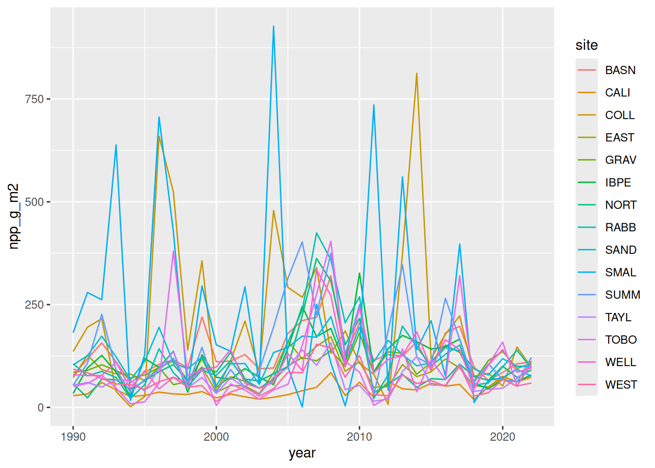
Now make a simple plot

g <- ggplot(data=anpp_data, aes(x=year, y=npp_g_m2, col=site)) + geom_line()

Show it

g

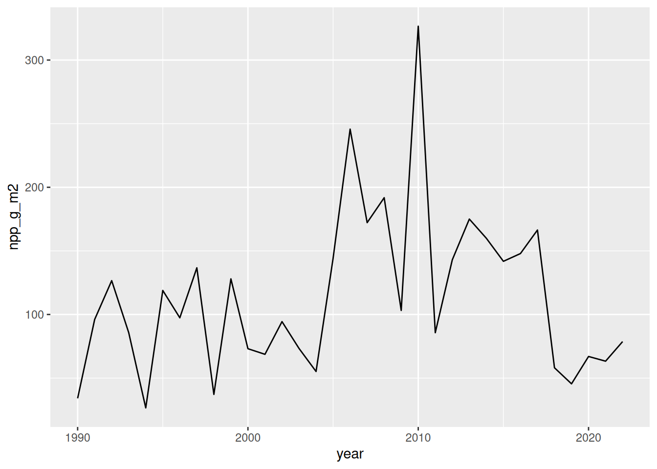
Now lets subset and plot site==IBPE

ibpe_anpp <- anpp_data |> filter(site==“IBPE”) g2 <- ggplot(data=ibpe_anpp, aes(x=year, y=npp_g_m2, col=site)) + geom_line()

g2

Set working directory to location where script is saved

#setwd(dirname(rstudioapi::getActiveDocumentContext()$path)) #dir(“data”)

Import total annual ANPP data

downloaded from https://portal.edirepository.org/nis/mapbrowse?scope=knb-lter-jrn&identifier=210011003

#anpp_data <- read_csv(“data/JRN011003_NPP_annual_site_summary.csv”)

Subset IBPE total ANPP data

#ibpe_anpp <- anpp_data %>% # dplyr::filter(site == “IBPE”)

Check avialble years

range(ibpe_anpp$year) # 1990 to 2022

Quick graph of the data

ggplot(ibpe_anpp, aes(x = year, y = npp_g_m2)) + geom_line()

Import shapefile of NPP sites

This can be downloaded from the Jornada Geoportal if you already

have access

NPP_sf <- st_read(“shp/Jornada_LTER_net_primary_production_study_sites_NPP_study_prj011__polygons.shp”)

Look at the columns of the data in the shapefile

glimpse(NPP_sf)

Subset IBPE site

IBPE_sf <- NPP_sf %>% dplyr::filter(site == “IBPE”) %>% st_transform(“EPSG:4326”)

Check coordinate reference system

st_crs(IBPE_sf)

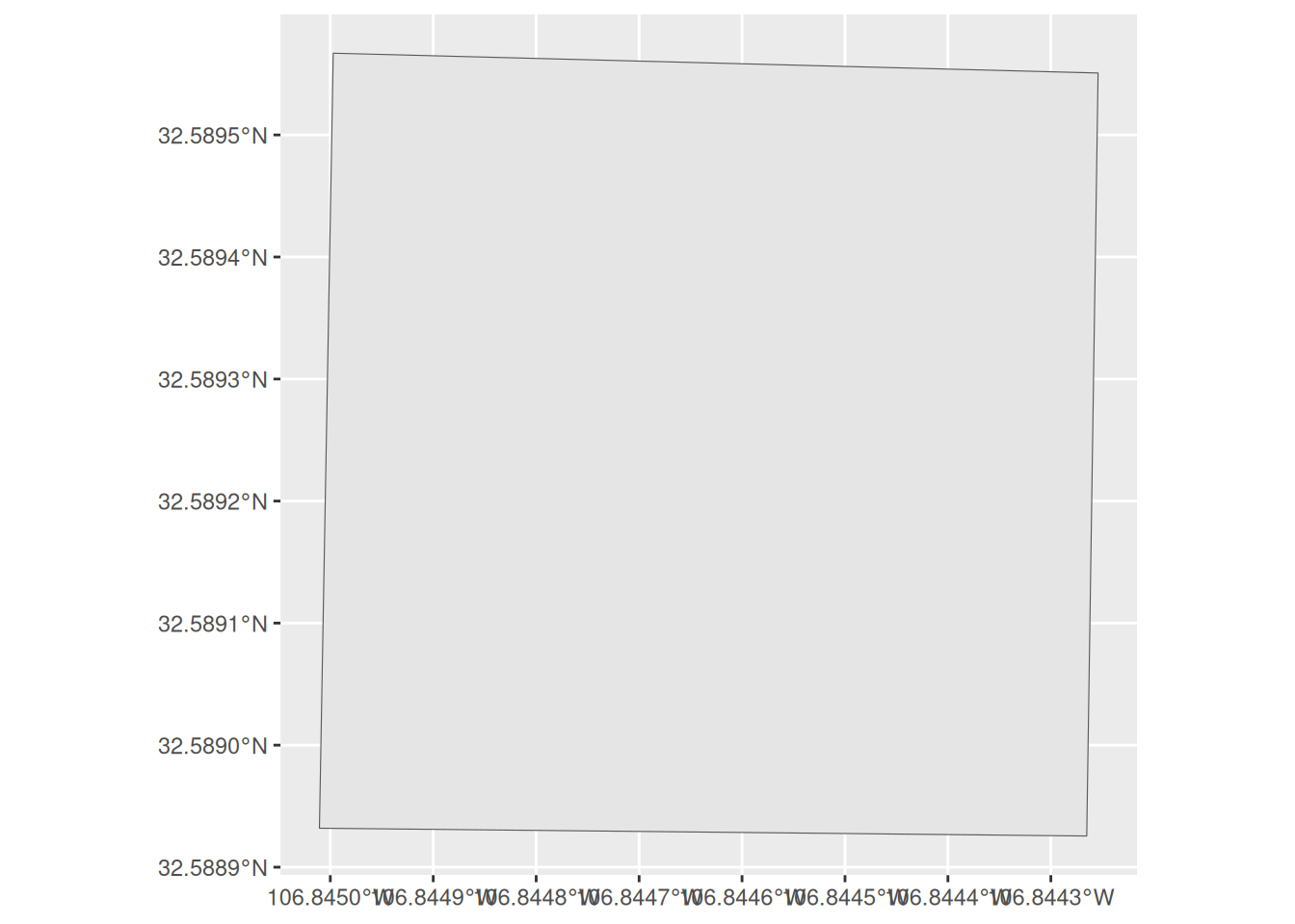
Quick figure of IBPE site polygon

ggplot(IBPE_sf) + geom_sf()

Use rapr::get_rap() function to access RAP data

Note that our shapefile is already in the “ESPG:4326” coordinate reference system

?get_rap

Currently, RAP biomass and production data are only available as a 30m pixel product

Each pixel is approximately 30m X 3m = 900m^2 in size

st_area(IBPE_sf) / 900 # The IBPE site is about 5.4 RAP pixels in size

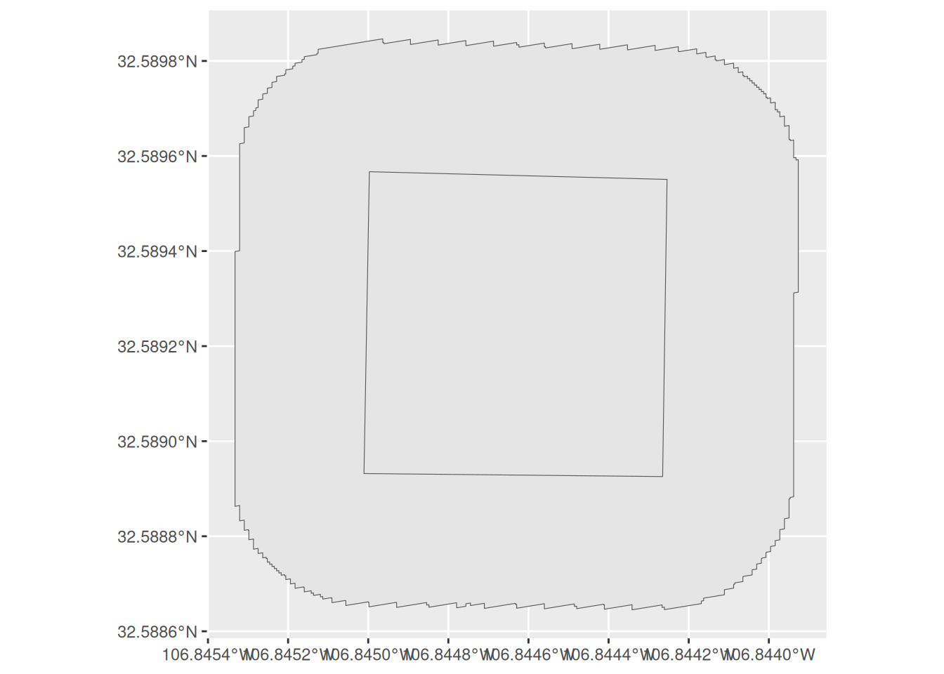
Buffer IBPE area by 30m to ensure complete coverage

Note that the LENGTHUNIT is already in meters

IBPE_buffer <- IBPE_sf %>% st_buffer(dist = 30)

Figure of IBPE site with 30m buffer

ggplot() + geom_sf(data = IBPE_buffer) + geom_sf(data = IBPE_sf)

Import 30m Landsat production data

IBPE_prod30m <- get_rap( x = IBPE_buffer, years = c(1990:2022), product = “vegetation-biomass”, source = “rap-30m”, sds = FALSE, verbose = TRUE )

Inspect the SpatRaster

IBPE_prod30m

Check the names

names(IBPE_prod30m)

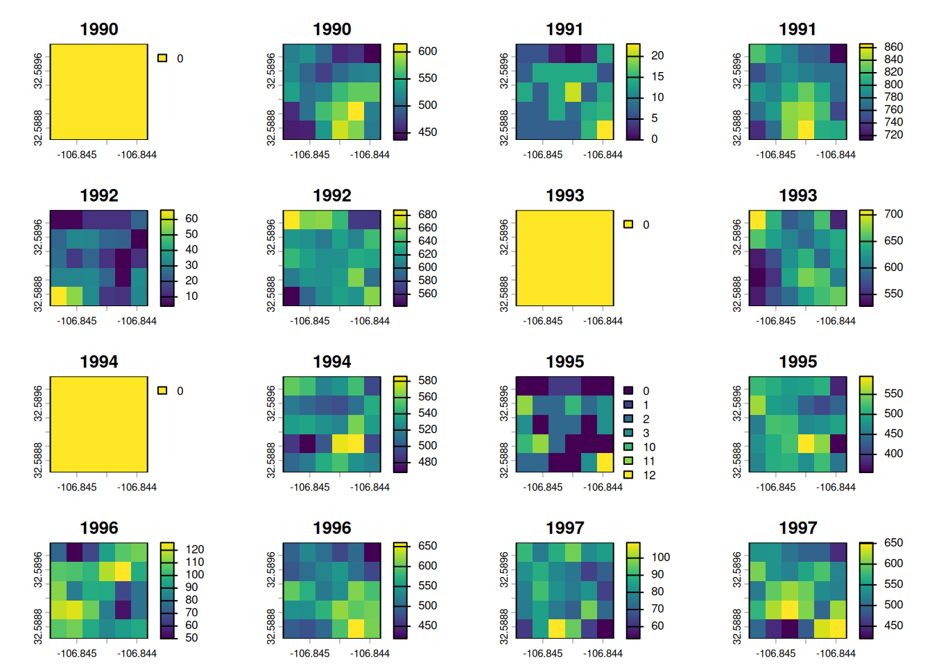
Use the default terra::plot() function to explore the data

Plots the first 16 rasters

plot(IBPE_prod30m)

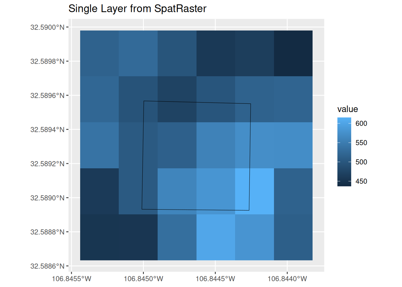
Graph the second raster with ggplot and geom_spatraster()

Overlay the IBPE site polygon

ggplot() + geom_spatraster(data = IBPE_prod30m[[2]]) + geom_sf(data = IBPE_sf, col = “black”, fill = NA) + labs(title = “Single Layer from SpatRaster”)

Use the terra::extract() function to calculate mean biomass at the IBPE site for each raster

Using exact = TRUE will caclualte a weigthed mean that uses partial pixels in the site boundary

Using exact = FALSE (default) will only use the pixels whose centroids are within the site boundary (4 pixels in this case)

rap_biomass_extract <- terra::extract(IBPE_prod30m, IBPE_sf, fun = “mean”, exact = TRUE)

Check the names of the extracted values

names(rap_biomass_extract)

Use tidyr::pivot_longer() to transpose the date from wide to long

rap_biomass_df <- rap_biomass_extract %>% pivot_longer(cols = starts_with(“vegetation”), names_to = “raster”, values_to = “biomass”)

Check the text strings of raster names

We need to find a way to extract the year from each of thes text strings

unique(rap_biomass_df$raster)

We can use the paste() function to construct a vector of all our years

separated by the “bar” symbol which functions as a n “OR” operator

paste(1990:2022, collapse = “|”)

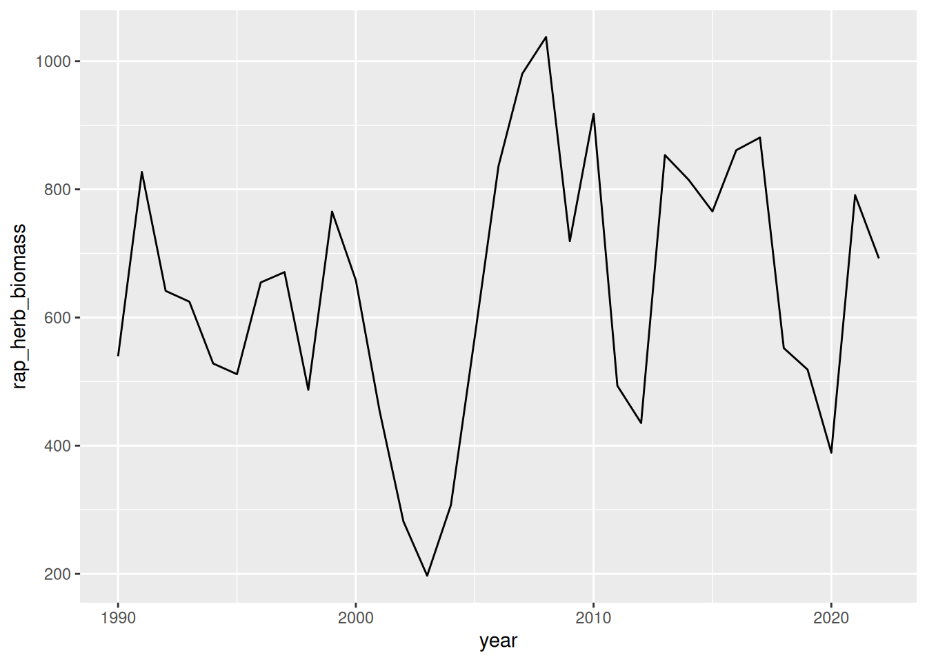
Use stringr::str_extract() to extract the year from the raster name, then covert to numeric

rap_biomass_df <- rap_biomass_extract %>% pivot_longer(cols = starts_with(“vegetation”), names_to = “raster”, values_to = “biomass”) %>% mutate(year = str_extract(string = raster, pattern = paste(1990:2022, collapse = “|”)) %>% as.numeric())

For each year, sum the biomass for annual forbs and grasses and perennial forbs and grasses

rap_biomass_year <- rap_biomass_df %>% group_by(year) %>% summarise(rap_herb_biomass = sum(biomass))

Quick plot of the data

ggplot(rap_biomass_year, aes(x = year, y = rap_herb_biomass)) + geom_line()

We want to join this data (by year) to the filed-based ANPP data

ibpe_anpp %>% left_join(rap_biomass_year)

Convert RAP from lbs/acre to grams/m^2

rap_biomass_convert <- rap_biomass_year %>% mutate(rap_g_m2 = rap_herb_biomass * 453.59237 / 4046.85642)

Now merge and transpose from wide to long

ibpe_biomass_merge <- ibpe_anpp %>% left_join(rap_biomass_convert %>% dplyr::select(year, rap_g_m2)) %>% pivot_longer(cols = c(npp_g_m2, rap_g_m2), names_to = “production_type”, values_to = “production_g_m2”)

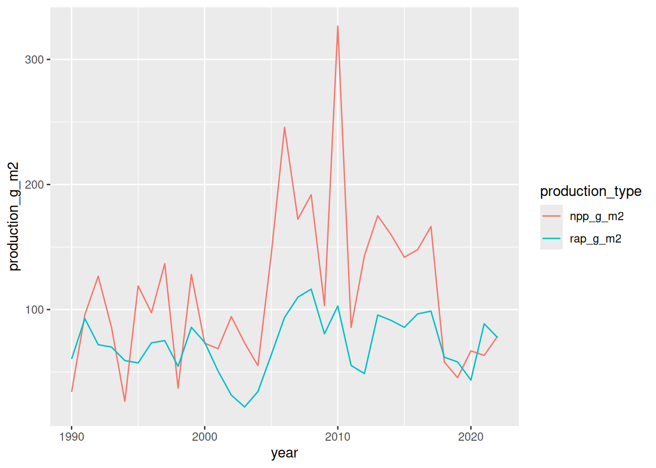
Quick graph of the data

ggplot(ibpe_biomass_merge, aes(x = year, y = production_g_m2, col = production_type)) + geom_line()

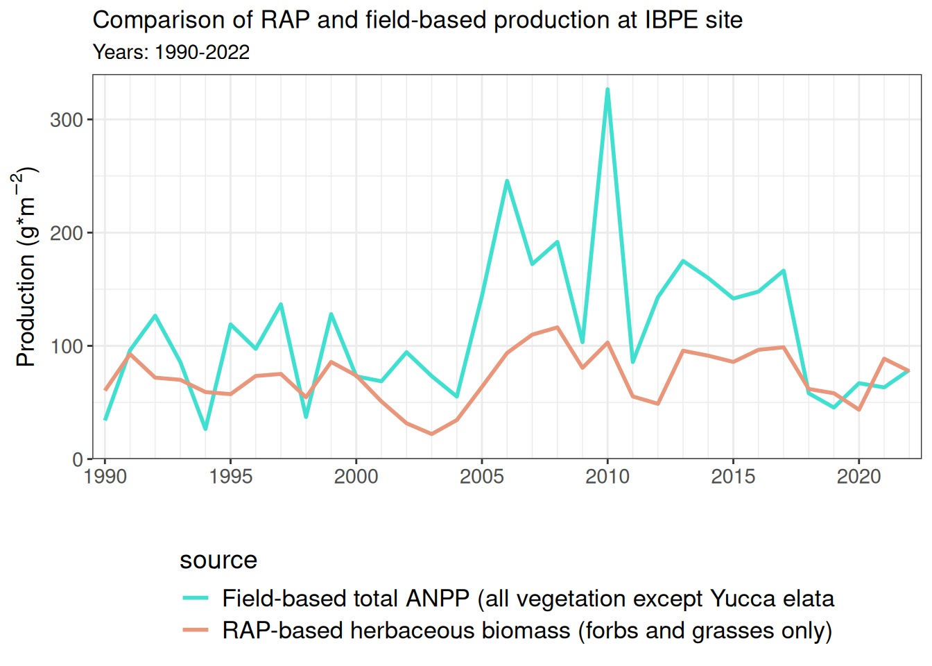
Make the graph prettier

ibpe_biomass_figure <- ibpe_biomass_merge %>% mutate(source = case_when(production_type == “npp_g_m2” ~ “Field-based total ANPP (all vegetation except Yucca elata”, production_type == “rap_g_m2” ~ “RAP-based herbaceous biomass (forbs and grasses only)”))

Check the range of the production values

range(ibpe_biomass_figure$production_g_m2)

ggplot(data = ibpe_biomass_figure, aes(x = year, y = production_g_m2, col = source)) + theme_bw() + geom_line(linewidth = 1) + scale_x_continuous(limits = c(1989.5, 2022.5), expand = c(0, 0), breaks = seq(from = 1990, to = 2022, by = 5), minor_breaks = 1990:2022) + theme(legend.position = “bottom”, legend.direction = “vertical”) + xlab(““) + ylab(bquote(”Production (g” m^-2 * “)”)) + ggtitle(“Comparison of RAP and field-based production at IBPE site”, subtitle = “Years: 1990-2022”) + theme(legend.title = element_text(size = 14), legend.text = element_text(size = 13)) + theme(axis.text = element_text(size = 11)) + theme(axis.title = element_text(size = 13)) + scale_color_manual(values = c(“turquoise”, “darksalmon”)) + scale_y_continuous(limits = c(0, 340), expand = c(0,0)) ````